2019, Dec 07
Recommending Movies
1. Motivation
During last years movie streaming platforms have become one of the most Internet services. Nowadays, everyone knows at least one of the biggest ones as for example Netflix.
In fact, all these streaming platforms provides thousands of movies and series for all the users. But, have you ever wondered how do they recommend you the perfect movies?

This jupyter notebook is going to help you with this question by creating two different recommender systems using the TMDB Movie Dataset and The Movies Dataset provided by Kaggle.
Besides these recommender systems are not going to be as complex as the Netflix one, they will show how recommender systems work in general.
2. Introduction to recommender systems
Recommender systems are defined as algorithms that try to produce recommendations of items according to different facts.
There exist different types of recommender systems, most common ones are based on finding the similarities between the elements we want to recommend or the users who use the recommender.
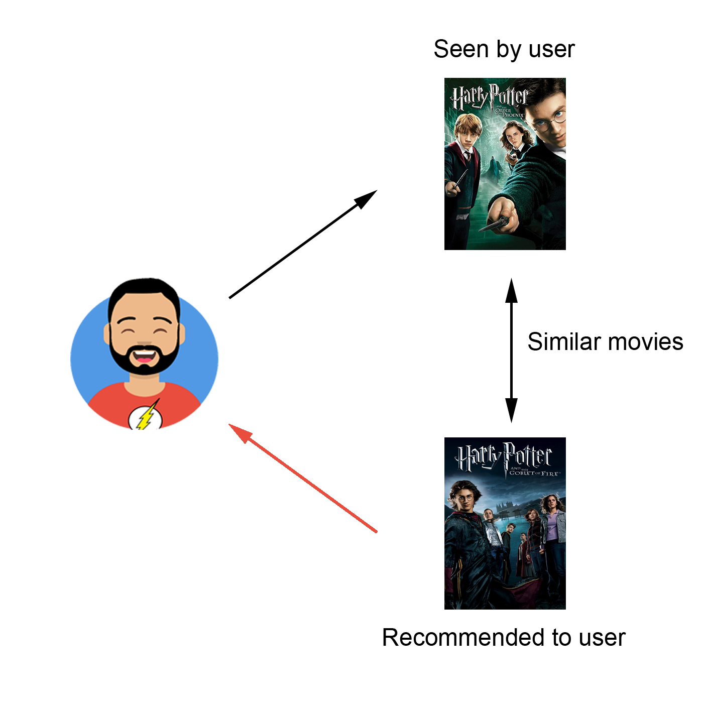
2.1. Content-based
When we talk about Content-based recommender systems, we refer to an algorithm where the recommendations are chosen by using the definitions of the elements that the user likes the most.
In other words, the attributes that define the elements are used to search for the most similar items. That is why this type of recommender system is named Content-based.
2.2. Collaborative-filtering
This type of recommender sytems use the ratings of the different users in order to predict which items should be recommended.
Collaborative-filtering analyzes the relation between users and creates a User-User similarity matrix. So, given a user, the recommended items are chosen according to what most similar users like.

3. Dependences
Before starting with data analysis, these are the main libraries used:
- pandas and numpy: all data vector and matrix operations.
- statistics: calculate some mathematical operations.
- sklearn: generation of tf-idf vectors and calculate cosine similarities.
- surprise: implementation of Collaborative-filtering model.
- ast: data processing.
- seaborn, wordcloud and matplotlib: visually plotting the obtained results.
- prettytable: result tables representation.
import statistics
import numpy as np
import pandas as pd
import seaborn as sns

import plotly.graph_objs as go
import plotly.express as px

from ast import literal_eval
from plotly.offline import iplot
from prettytable import PrettyTable
from matplotlib import pyplot as plt
from wordcloud.wordcloud import WordCloud

from sklearn.metrics.pairwise import cosine_similarity
from sklearn.feature_extraction.text import TfidfVectorizer

from surprise import Reader, Dataset, SVD
from surprise.model_selection import cross_validate
4. Data exploration
Before analyzing our datasets, we should first familiarize with our data in order to understand the data we have.
# We load both datasets
movies_path = r"./Data/tmdb_5000_movies.csv"
movies = pd.read_csv(movies_path)

ratings_path = r"./Data/ratings_small.csv"
ratings = pd.read_csv(ratings_path)
ratings = ratings[ratings['movieId'].isin(movies.index.values)]
First of all, we are going to start by exploring the movies dataset.
# We print the movies dataset shape
print("Number of movies:", movies.shape[0], '.')
print("Attributes per movie:", movies.shape[1], '.')
As we can appreciate, we have over 4800 movies and 20 attributes for each one.
The following table shows a few examples where we can watch all the attributes we have.
pd.set_option("display.max_columns", None)
movies.head(3)
If we observe these examples we can see that for each movie we have a lot of information: genres, keywords, budget, runtime, etc.
But, are we sure that movies instances include all these attributes? In order to verify this, next step is searching for missing values:
na_table = PrettyTable()
na_table.field_names = ["Attribute", "Missing values count", "Missing value percentage (by attribute)"]

for attribute in movies.columns:
    na_count = pd.isna(movies[attribute]).sum()
    na_percentage = round(na_count / movies.shape[0], 2)
    if na_count > 0:
        na_table.add_row([attribute, na_count, na_percentage])

print(na_table)
If we observe this table we can see how two attributes have a lot of missing values. These missing values should be processed to avoid different issues when developing our model. However, this time there is no need for processing them since none of these specific attributes are going to be used later.
Once we have explore our movies data, it is time to do the same with the ratings.
# We print the ratings dataset shape
print("Number of user ratings:", ratings.shape[0], '.')
print("Attributes per user rating:", ratings.shape[1], '.')
Now lets take a look on a few user rating examples:
ratings.head()
As we can appreciate, for each user rating we have the relation between the user and the movie rated. Moreover, there is also the rating in a 5-point scale and a timestamp that gives us information about when this rating has been done.
Next step is searching for missing values:
na_table = PrettyTable()
na_table.field_names = ["Attribute", "Missing values count"]

for attribute in ratings.columns:
    na_counts = pd.isna(ratings[attribute]).sum()
    na_table.add_row([attribute, na_count])

print(na_table)
We can confirm that there are no missing values in the ratings dataset.
5. Data analysis
Before starting with the data analysis we are going to restructure some attributes in a simpler and more efficient way.
This reestructarization consists in representing the complex attributes with simplier lists.
for attribute in ['genres', 'keywords', 'production_companies', 'production_countries']:
    movies[attribute] = movies[attribute].fillna('[]')
    movies[attribute] = movies[attribute].apply(literal_eval)
    movies[attribute] = movies[attribute].apply(lambda x: [i['name'] for i in x] if isinstance(x, list) else [])

movies['spoken_languages'] = movies['spoken_languages'].fillna('[]')
movies['spoken_languages'] = movies['spoken_languages'].apply(literal_eval)
movies['spoken_languages'] = movies['spoken_languages'].apply(
    lambda x: [i['iso_639_1'] for i in x] if isinstance(x, list) else [])
One attribute that can be intresting is which are the spoken languages of the movies. For this, we are going to plot the 10 most spoken languages in all the movies:
# We count how many times a each language is spoken in a movie.
languages_count = dict()
for languages, count in movies['spoken_languages'].apply(tuple).value_counts().iteritems():
    for language in languages:
        if language in languages_count.keys():
            languages_count[language] += count
        else:
            languages_count[language] = count

# We sort the languages according to their count value and select the 10 first ones.
languages = pd.DataFrame({'language':list(languages_count.keys()), 'count':list(languages_count.values())})
languages = languages.sort_values('count', ascending=False)
languages = languages.head(10)

# We represent the languages by using a pie chart.
# colors = ['#0077B6', '#00B4D8', '#90E0EF', '#CAF0F8', '#03045E', '#045797', '#27D0FE', '#1A3763', '#A4C0EA']

labels = languages['language'].values.tolist()
values = languages['count'].values.tolist()

trace = go.Pie(labels=labels,
               values=values,
               textinfo='label+percent',
               hole=0.3)

data = [trace]

figure = go.Figure(data)
figure.update_layout(title="Spoken Languages Proportions", width=900, height=400)

iplot(figure)
As expected, the most spoken language in all the movies is English.
Now, lets take a look on the movies genres and try to know which genres are more frequent:
def select_color(word=None, font_size=None, position=None, orientation=None, font_path=None, random_state=None):
    return "hsl(275, 100%," + str(random_state.randint(20, 65)) + "%)"

def plot_word_cloud(attribute, n=None):
    frequency = dict()
    for values, num in movies[attribute].apply(tuple).value_counts().iteritems():
        for value in values:
            if value in frequency.keys():
                frequency[value] += num
            else:
                frequency[value] = num
    frequency = {k: v for k, v in sorted(frequency.items(), key=lambda item: item[1], reverse=True)[:n]}
    wc = WordCloud(width=1920, height=1080, background_color='white', color_func=select_color)
    word_cloud = wc.generate_from_frequencies(frequency)
    plt.figure(figsize=(10,5))
    plt.imshow(word_cloud, interpolation='bilinear')
    plt.axis("off")
    plt.show()


plot_word_cloud('genres')

This wordcloud represents the most frequent genres in the dataset by using the size of each word. So, the bigger the word is, the more frequent it is. As we can see, Drama and Comedy are the most frequent movie genres in our data.
Another intresting fact to know is which keywords are more frequent in our data. In order to analyze that fact, we are going to create another wordcloud but with all the keywords we have:
plot_word_cloud('keywords')

In this word cloud we can observe how there are a lot of keywords. The most frequent ones are for example: "Independent film" or "Woman director".
Now, it would be intresting to see which movies have been rated the most.
times_rated = pd.DataFrame({'movieId':ratings['movieId'].value_counts().head(10).index.values,
                            'count':ratings['movieId'].value_counts().head(10).values})

times_rated['movieTitle'] = times_rated['movieId'].apply(lambda x: movies.loc[x]['title'])

figure = px.bar(times_rated, x='count', y='movieTitle', color='movieTitle', orientation='h')

figure.update_layout(title="Most rated movies",
                     xaxis=dict(title="Count"),
                     yaxis=dict(title="Movie"),
                     legend_title_text='Movies',
                     width=900,
                     height=300)

iplot(figure)
This plot represents the number of ratings that a movie has. As we can see, "Sherlock Holmes" is the most rated movie in our data.
Once we know which movies have been rated the most, it would be great to take a look at the number of non-rated movies:
rated_movies = ratings['movieId'].unique()
non_rated_movies = list(filter(lambda x: x not in rated_movies, movies.index.values))
print("A", round(100 * len(non_rated_movies) / movies.shape[0], 2),
      "% of the movies have no ratings (" + str(len(non_rated_movies)) + " of " + str(movies.shape[0]) + ").")
This information we have just seen is very important for when we try to create a collaborative-filtering recommender system. It tells us that a lot of movies will not be possible to be recommended when using this type of recommender system since nobody has rated them.
On the other hand, it would be great to know how many movies are rated per user.
plt.figure(figsize=(15,5))
kwargs = {'cumulative': True}
ax = sns.distplot(ratings["userId"].value_counts(), hist_kws=kwargs, kde_kws=kwargs)
ax.set(xlabel="Maximum number of ratings", ylabel="Users percentage")
plt.xticks(np.arange(0, max(ratings["userId"].value_counts()) + 1, 100))
plt.show()

If we observe this accumulative histogram we can see how approximately an 90% of the users with ratings have 200 or less. This is normal since 200 ratings are a lot for a single user.
6. Data preparation
During the analysis of the movies dataset, we have seen a lot of attributes and instances containing missing values. However, we are not going to process them this time, but just because these attributes are not going to be used in our recommender system.
First of all, we are going to create some helpful functions that will be used later:
get_movie_idx: given a movie title this function returns its index in the movies dataframe.
get_movie_title: given a movie id this funcion returns its title.
get_movies_rated: this function returns a DataFrame with all the ratings of the given a user.
def get_movie_idx(movie_title):
    movie_idx = movies.index[movies['title'] == movie_title].to_list()
    if movie_idx:
        return movie_idx[0]
    else:
        return None

def get_movie_title(movie_id):
    if movie_id in movies.index.values:
        return movies.loc[movie_id]['title']
    else:
        return None

def get_movies_rated(user_id):
    movies_rated = ratings[ratings['userId'] == user_id][['movieId', 'rating']]
    movies_rated['movieTitle'] = movies_rated['movieId'].apply(get_movie_title)
    movies_rated = movies_rated.sort_values('rating', ascending=False)
    movies_rated = movies_rated[['movieTitle', 'movieId', 'rating']].set_index(
        "movieTitle")
    return movies_rated
Also, we are going to add to the ratings one more attribute containing the title of the movie.
ratings['movieTitle'] = ratings['movieId'].apply(get_movie_title)
7. Model creation
7.1. Content-based
For this type of recommender system we need to select only the attributes that better represents the content of each movie. So, after taking a look on our possible attributes, we have selected the ones below:
- Keywords.
- Genres.
- Spoken languages.
First step is to join them in order to use them for calculating the similarities between movies:
selected_attributes = ['genres', 'keywords', 'spoken_languages']

movies_info = pd.Series(movies[selected_attributes].values.tolist(), index=movies.index.values).apply(
    lambda x: ' '.join(x[0] + x[1] + x[2]))
Once collected all the descriptive words fot each movie, lets see how this information is stored:
movies_info.head()
As we can see, all the words for each movie are stored in his own row.
Before doing the next step, we first need to understand what does tf-idf means.
Tf-idf (Term frequency - inverse document frequency) is used to evaluate how important a word is to a "document" in a collection or corpus.
This weight is compute by two terms:
Term Frequency (TF): The first one computes the number of times a word appears in a specific document divided by the total number of words in that document.
Inverse Document Frequency (IDF): Measures how important a word is by computing the logarithm of the number of documents in the corpus divided by the number of documents where this specific word appears.
Once calculated both terms, the weight is obtained by computing the product.
Example:
We have a document that contains 100 words where the word "movie" appears 5 times. Then, the term frequency (TF) for "movie" is: 5/100 = 0.05.
Now, lets assume that we have a corpus of 20000 documents where the words "movie" appears in 100 of them. So, the inverse document frecuency (IDF) is: log(20000/100) = 2.3.
Then the tf-idf weight is: 0.05 * 2.3 = 0.115.
Stop words are another important and useful concept when computing the tf-idf vector. These words do not have a meaning by themselves, they only modify or accompany others. This is why stop words are usually composed of articles, pronouns, prepositions, adverbs, and more.
So, as we do not want meaningless information, we specify that stop words are filtered before generating the tf-idf vectors.
tfidf_vectorizer = TfidfVectorizer(stop_words='english')
tfidf = tfidf_vectorizer.fit_transform(movies_info)
After the tf-idf vectors have been generated, the next step is to calculate the similarity between movies by using these tf-idf vectors.
In order to calculate the similarity between movies, we are using the cosine similarity.
cosine_similarity = cosine_similarity(tfidf, tfidf)
Now we have all the necessary to create a function that, given a title, returns the n most similar movies.
def similar_movies(title, n=10):
    movie_id = get_movie_idx(title)
    if movie_id is None:
        print("Movie not found.")
    else:
        movie_similarities = sorted(list(enumerate(cosine_similarity[movie_id])), key=lambda x: x[1], reverse=True)
        most_similar_movies = list(map(lambda x: (get_movie_title(x[0]), round(x[1], 2)), movie_similarities[:n+1]))
        most_similar_movies = list(filter(lambda x: title != x[0], most_similar_movies))

        recommended_movies = PrettyTable()
        recommended_movies.field_names = ["Movie", "Cosine Similarity"]
        for movie_title, similarity in most_similar_movies:
            recommended_movies.add_row([movie_title, similarity])
        print(recommended_movies)
Once the function has been defined, we can try to see which movies are similar to a chosen one to test how it works:
similar_movies('Avatar')
As we can see, the function shows the 10 most similar movies to Avatar. If we take a look all of them have a lot of similarities as for example being a space-theme movie.
7.2. Collaborative-filtering
Now it is time to implement the collaborative-filtering. As we have commented before, the similarity between uses is the main core of this type of recommender systems.
In the Data analysis we have came up with two important facts:
- A lot of movies have no ratings.
- There are users with a few ratings.
First of all, we are going to filter the users that have less than a certain number of ratings:
users_before = ratings['userId'].value_counts().shape[0]

min_ratings_per_user = 40
ratings = ratings[ratings['userId'].map(ratings['userId'].value_counts()) > min_ratings_per_user]

users_now = ratings['userId'].value_counts().shape[0]

print("The number of users has been reduced to", users_now, "from", users_before)
As we can see the number of users has been reduced a lot. Now, lets filter the movies that have less than a minimum number of ratings:
movies_before = ratings['movieId'].value_counts().shape[0]

min_ratings_per_movie = 100
ratings = ratings[ratings['movieId'].map(ratings['movieId'].value_counts()) > min_ratings_per_movie]

movies_now = ratings['movieId'].value_counts().shape[0]

print("The number of rated movies has been reduced to", movies_now, "from", movies_before)
Once filtered our ratings data, it is time to create a SVD model. The Singular-Value Decomposition (SVD), is a matrix decomposition method for reducing a matrix to its constituent parts in order to make certain subsequent matrix calculations simpler.
svd = SVD()
Now is time to evaluate it by using k-fold:
reader = Reader()
data = Dataset.load_from_df(ratings[["userId", "movieId", "rating"]], reader)

results = cross_validate(svd, data, measures=['RMSE', 'MAE'], cv=5)

mae_results = list(map(lambda x: round(x, 2), results['test_mae']))
mae_mean = round(statistics.mean(mae_results), 2)
mae_std = round(statistics.stdev(mae_results), 4)

rmse_results = list(map(lambda x: round(x, 2), results['test_rmse']))
rmse_mean = round(statistics.mean(rmse_results), 2)
rmse_std = round(statistics.stdev(rmse_results), 4)

results_table = PrettyTable()
results_table.field_names = ["Metric","Fold 1", "Fold 2", "Fold 3", "Fold 4", "Fold 5", "Mean", "Std"]
results_table.add_row(["MAE"] + mae_results + [mae_mean, mae_std])
results_table.add_row(["RMSE"] + rmse_results + [rmse_mean, rmse_std])

print(results_table)
As we can see, we have reached a really good RMSE value and the MAE value is also quite good.
Next step is fitting our SVD model.
train_set = data.build_full_trainset()
svd = svd.fit(train_set)
Once our model has been fitted, we can try to estimate the rating of the rated movies of a user in order too observe how it works:
user_id = 2

movies_rated = get_movies_rated(user_id)

movies_rated['prediction'] = movies_rated['movieId'].apply(lambda x: svd.predict(user_id, x).est)

print(movies_rated.sample(10))
We need to create a function that given a user identifier, returns the recommended movies:
def recommend_movies(user_id, n=10):

    seen = get_movies_rated(user_id)['movieId'].to_list()

    not_seen = list(set(ratings[~ratings['movieId'].isin(seen)]['movieId'].to_list()))

    predicted_movies = pd.DataFrame(not_seen, columns=['movieId'])

    predicted_movies['movieTitle'] = predicted_movies['movieId'].apply(get_movie_title)

    predicted_movies['prediction'] = predicted_movies['movieId'].apply(lambda x: svd.predict(user_id, x).est)

    predicted_movies = predicted_movies.sort_values('prediction', ascending=False)

    predicted_movies = predicted_movies[["movieTitle", "prediction"]]

    predicted_movies = predicted_movies.set_index("movieTitle")

    print(predicted_movies.head(n))
Before trying our collaborative-filtering model, lets see the 10 most rated movies of the user:
ratings[ratings["userId"] == user_id].sort_values("rating", ascending=False).head(10)[["movieTitle", "rating"]]
Now, lets try our collaborative-filtering model:
recommend_movies(user_id, 10)
These results are difficult to evaluate because the recommendations are based on the similarities between users and it is not as simple as checking if the movies are similar.
8. Conclusions
After all the analysis and the results obtained, we can expose the following conclusions:
- We have been able to implement two different types of recommender systems for our collections of users and movies.
- The Content-based implementation achieves good results when searching for similar movies.
- When implementing a Collaborative-filtering recommender system we need to be careful about two important things:
- The number of ratings per user.
- The number of ratings of a movie.
- A Collaborative-filtering method requires a lot of ratings.