2020, Mar 07
How to start classifying with TensorFlow 2.0
1. Introduction
If you don't know how to start creating a classifier, and how to use TensorFlow, this article will be especially dedicated to solving this question.
We are going to use the dataset Intel Image Classification from Kaggle to do a tutorial for how to start with TensorFlow and how to create a classifier, looking for the best accuracy. This dataset contains images of Natural Scenes aroung the world and there are around 25K images distributed under 6 categories as we are going to see.
As an outline for this article, the following topics will be covered:
- How to start with TensorFlow 2.0
- CNN Model
- Apply Data Augmentation techniques
- Fine-Tuning with MobileNetV2
1.1. How to start with TensorFlow 2.0
What is TensorFlow?
TensorFlow is a machine learning framework that Google created to design, build, and train deep learning models. It has an excellent balance of flexibility and scalability.
TensorFlow consists of APIs at different levels. At the highest level, we have the Estimators that make it easy to develop a Machine Learning pipeline, and also we have Keras, a friendly API to create and train neural networks.
This is the API that we will use in this Blogspot. If you want to know more about how works TensorFlow you can check the documentation.
First of all, you have to install it and you will see some of the most common ways on the TensorFlow installation webpage. Once you have installed it, you can now import it to the workspace as you can see in the bellow cell.
# Imports
import tensorflow
from tensorflow.keras.preprocessing.image import ImageDataGenerator
from tensorflow.keras.callbacks import EarlyStopping
from tensorflow.keras.models import Sequential
from tensorflow.keras.layers import Conv2D, GlobalAveragePooling2D, MaxPool2D, Dense, Flatten, Dropout
from tensorflow.keras.optimizers import RMSprop
from tensorflow.keras.applications import MobileNetV2
from keras.preprocessing import image
import os
import pathlib
import numpy as np
import matplotlib.pyplot as plt
1.2. Data Information
Now we are going to see how many images and classes we have in the dataset.
train_dir = pathlib.Path("/content/intel_image/seg_train/seg_train/")
test_dir = pathlib.Path("/content/intel_image/seg_test/seg_test/")
print("We have ", len(list(train_dir.glob('*/*.jpg'))), "images in train set.")
print("We have ", len(list(test_dir.glob('*/*.jpg'))), "images in test set.")
class_names = list([item.name for item in train_dir.glob('*')])
print("We have the following classes:", class_names)
1.3. Image Data Generator
As we said before, we are going to use the preprocessing tool from Keras. We will use the ImageDataGenerator that generate batches of tensor image data to load the dataset.
To use this generator function from Keras, we must have the images in a specific directory format:
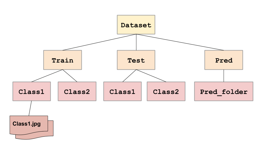
The constructor for the ImageDataGenerator contains many arguments to specify how to manipulate the image data after it is loaded, but for now, we only configure it with the rescale parameter to convert from uint8 to float32 in the range [0,1].
Then, we have to call the _flow_from_directory()_ function to specify the dataset directory such as the train and test directory.
Also, we can configure more details such as:
- _Target_size_ that allows us to load all images to a specific size, which in our case is going to be 150x150.
- _Batchsize that is going to be 32, which means that 32 randomly selected images from across the classes in the dataset will be returned in each batch when training.
- _Classmode to specify the type of classification task. In our case a multi-class classification: 'categorical'.
image_generator = ImageDataGenerator(rescale=1./255)

train_generator = image_generator.flow_from_directory(train_dir,
                                                      target_size = (150,150),
                                                      batch_size=32,
                                                      class_mode='categorical')

test_generator = image_generator.flow_from_directory(test_dir,
                                                     target_size=(150,150),
                                                     batch_size=32,
                                                     class_mode='categorical')
1.4 Data Exploration
We are going to create a simple function to show some random images of our dataset.
def show_batch(image_batch, label_batch):
    plt.figure(figsize=(10,10))
    for n in range(10):
        ax = plt.subplot(5,5,n+1)
        plt.imshow(image_batch[n])
        plt.title(np.array(class_names)[label_batch[n]==1][0].title())
        plt.axis('off')
image_batch, label_batch = next(train_generator)
show_batch(image_batch, label_batch)

2. Creating a simple Neural Network
We are going to create a very simple neural network to understand how to train and evaluate it with TensorFlow.
Before starting, we have to understand the meaning of Early Stopping: it is a method that allows us to specify an arbitrarily large number of training epochs and stop training once the model performance stops improving on a held out validation dataset.
Keras supports the early stopping of training via a callback called EarlyStopping. So we are going to configure it with the next parameters: monitor that allows us to specify the performance measure to monitor in order to end training, and patience to define the number of epochs on which we would like to see no improvement.
early_stopping = EarlyStopping(monitor='val_loss', patience=3)
Now, its time to build the model by stacking layers.
# Create model adding different layers.
# Using 'softmax' activation because we have a multiclass classification.
model = Sequential([Flatten(),
                    Dense(512, activation = 'relu'),
                    Dense(256, activation = 'relu'),
                    Dropout(rate=0.5),
                    Dense(6, activation = 'softmax')])

# Compile the model
# loss: categorical_crossentropy because the targets are one-hot encoded.
model.compile(optimizer='adam',
              loss='categorical_crossentropy',
              metrics=['accuracy'])
Once we are here, fitting the model can be achieved by calling the next function passing the training and test set. Also, we can pass the verbose argument that allows us to discover the training epoch on which training was stopped.
# Fitting the model training with train test and validate test set.
# Callback: early_stopping
trained_MLP = model.fit(train_generator,
                    validation_data  = test_generator,
                    epochs = 50,
                    verbose = 1,
                    callbacks= [early_stopping]);

# Save weights
model.save_weights('weights_MLP.h5')
Now we are going to create a function to plot the accuracy and the loss over the epochs.
def plot_acc_loss(trained):
    fig, ax = plt.subplots(1, 2, figsize=(15,5))
    ax[0].set_title('loss')
    ax[0].plot(trained.epoch, trained.history["loss"], label="Train loss")
    ax[0].plot(trained.epoch, trained.history["val_loss"], label="Validation loss")
    ax[1].set_title('acc')
    ax[1].plot(trained.epoch, trained.history["accuracy"], label="Train acc")
    ax[1].plot(trained.epoch, trained.history["val_accuracy"], label="Validation acc")
    ax[0].legend()
    ax[1].legend()
plot_acc_loss(trained_MLP)

The model.evaluate method checks the models performance, on the test set.
#Loading weights
model.load_weights('weights_MLP.h5')

# Evaluate the model with the test set.
model_MLP_score = model.evaluate(test_generator)
print("Model MLP Test Loss:", model_MLP_score[0])
print("Model MLP Test Accuracy:", model_MLP_score[1])
3. CNN Model
Now that we have seen how to create and train a basic neural network, we are going to introduce a Convolutional Neural Network.
Why are we going to use it?
Because MLPs do not scale well for images and also ignore the information brought by pixel position and correlation with neighbors. Instead, CNN are mostly used for image processing and classification because they can handle the limitations of MLPs.
We will not go into depth on how they work internally since it is out of the scopte of this blog. You can find an article in this Blog with all the information: Introduction to CNN.
The CNN architecture that we will use is a simple one, to see if improves our Accuracy. There are going to be the next layers:
- Conv2D with 200 filters of size 3 by 3. These layers are responsible for extracting features from the image.
- MaxPool2D to reduce the spatial volume of input image after a convolution.
- Fully Connected Layer to connect the network from a layer to another one.
# Create the model adding Conv2D.
model = Sequential([Conv2D(200, (3,3), activation='relu', input_shape=(150, 150, 3)),
                    MaxPool2D(5,5),
                    Conv2D(180, (3,3), activation='relu'),
                    MaxPool2D(5,5),
                    Flatten(),
                    Dense(180, activation='relu'),
                    Dropout(rate=0.5),
                    Dense(6, activation='softmax')])

# Compile model.
# Loss categorical_crossentropy: targets are one-hot encoded.
model.compile(optimizer='adam',
              loss='categorical_crossentropy',
              metrics=['accuracy'])
# Fitting the model training with train test and validate test set.
# Callback: early_stopping
trained_CNN = model.fit(train_generator,
                    validation_data  = test_generator,
                    epochs = 40,
                    verbose = 1,
                    callbacks= [early_stopping]);

# Save weights
model.save_weights('weights_CNN.h5')
plot_acc_loss(trained_CNN)

# Load weights and evaluate model
model.load_weights('weights_CNN.h5')
model_CNN_score = model.evaluate(test_generator)
print("Model CNN Test Loss:", model_CNN_score[0])
print("Model CNN Test Accuracy:", model_CNN_score[1])
6. Apply Data Augmentation
Image data augmentation is a technique that can be used to artificially expand the size of the training set by creating modified versions of images in the dataset in order to reduce overfitting.
Keras provides us the capability to fit our models using image data augmentation via the ImageDataGenerator that we saw earlier.
A brief explication of each parameter that we will use:
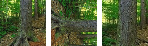
- Shear_range: for randomly applying shearing transformations.
- Zoom_range: for randomly zooming inside pictures.
- Horizontal_flip: for randomly flipping half of the images horizontally.
For example, if we flip this image of a tree, you still know that it is a tree and if you zoom this picture, too.
# Create ImageDataGenerator with new parameters for Data Augmentation
image_generator = ImageDataGenerator(
    rescale=1./255,
    shear_range=0.2,
    zoom_range=0.2,
    horizontal_flip=True,
    validation_split=0.3)
train_generator = image_generator.flow_from_directory(train_dir,
                                                      target_size = (150,150),
                                                      batch_size=32,
                                                      shuffle=True,
                                                      seed=10,
                                                      class_mode='categorical')

test_generator = image_generator.flow_from_directory(test_dir,
                                                     target_size=(150,150),
                                                     batch_size=32,
                                                     shuffle=True,
                                                     seed=10,
                                                     class_mode='categorical')
# Create the same model as the previous one
model = Sequential([Conv2D(200, (3,3), activation='relu', input_shape=(150, 150, 3)),
                    MaxPool2D(5,5),
                    Conv2D(180, (3,3), activation='relu'),
                    MaxPool2D(5,5),
                    Flatten(),
                    Dense(180, activation='relu'),
                    Dropout(rate=0.5),
                    Dense(6, activation='softmax')])

model.compile(optimizer='adam',
              loss='categorical_crossentropy',
              metrics=['accuracy'])
# Fitting the model training with train test and validate test set.
# Callback: early_stopping
trained_DA = model.fit(train_generator,
                    validation_data  = test_generator,
                    epochs = 40,
                    verbose = 1,
                    callbacks= [early_stopping])

# Save weights
model.save_weights('weights_CNN_DA.h5')
plot_acc_loss(trained_DA)

# Load weights and evaluate model
model.load_weights('weights_CNN_DA.h5')
model_DA_score = model.evaluate(test_generator)
print("Model with Data Augmentation Test Loss:", model_DA_score[0])
print("Model with Data Augmentation Test Accuracy:", model_DA_score[1])
7. Fine tuning
Now that we have seen how to create a CNN model, and how to do data augmentation and observe the results, we are going to fine-tune a popular network model: MobileNet.
What is Fine Tuning?
First of all, we have to know that Fine-tuning is a way of applying transfer learning.
Transfer learning occurs when we use the knowledge that was gained from solving one problem and apply it to a new but related problem. So, as we said, fine-tuning is a way of utilizing it.
It is a process that takes a model that has already been trained for one given task and then tunes the model to make it perform a second similar task.
![]()
Why are we going to use Fine-Tuning?
Usually, we are going to use it when we have a task that is similar to a model that has already been designed and trained, allowing us to take advantage of that without having to develop it from scratch. Also when you have a small amount of data for the new problem compared with the previous one.
We are going to use the MobileNetV2 network, that it's faster and smaller than other major networks, like VGG16.
mobile_model = MobileNetV2(input_shape=(150, 150,3), include_top=False, weights='imagenet')

mobile_model.trainable = True

print("Number of layers in the MobileNetV2 model: ", len(mobile_model.layers))
We are going to un-freeze some of the layers that in the pre-trained model is close to the top because lower convolutional layers detects low-level features like edges and curves, while the higher level, which is more specialized, detect features that are applicable to our problem (As can be seen in the diagram above).
fine_tune_at = 100
for layer in mobile_model.layers[:fine_tune_at]:
    layer.trainable =  False
The last layer of the MobileNetV2 has the output shape: (input width = 5) x (input height = 5) x (input channels = 1280). That is why we are going to use the GlobalAveragePooling2D, because it takes this tensor and computes the average value of all values across the entire (input width) x (input height) matrix for each of the input channels.

So, the output it's going to be a 1-dimensional tensor of the size of the input channels as we can see in the summary.
# Create model adding the pre-trained model mobileNetV2,
# adding GlobalAveragePooling2D layer
model = Sequential([mobile_model,
                    GlobalAveragePooling2D(),
                    Dropout(rate=0.5),
                    Dense(6, activation='softmax')])

model.compile(optimizer= RMSprop(lr=2e-5),
              loss='categorical_crossentropy',
              metrics=['accuracy'])

model.summary()
# Fitting model and save weights
trained_FT = model.fit(train_generator,
                    epochs=20,
                    validation_data=test_generator,
                    callbacks=[early_stopping])

model.save_weights('weights_FT.h5')
plot_acc_loss(trained_FT)

model.load_weights('weights_FT.h5')
model_FT_score = model.evaluate(test_generator)
print("Model Fine Tuning Test Loss:", model_FT_score[0])
print("Model Fine Tuning Test Accuracy:", model_FT_score[1])
We can plot some images from the prediction set to predict the classes.
img1 = image.load_img('/content/intel_image/seg_pred/seg_pred/5.jpg', target_size=(150, 150))
x = image.img_to_array(img1)
x = np.expand_dims(x, axis=0)
prediction1 = model.predict(x, batch_size=10)

img2 = image.load_img('/content/intel_image/seg_pred/seg_pred/176.jpg', target_size=(150, 150))
y = image.img_to_array(img2)
y = np.expand_dims(y, axis=0)
prediction2 = model.predict(y, batch_size=10)

plt.figure()
plt.subplot(121)
plt.title("Predicted class: " + str(np.argmax(prediction1[0])))
plt.imshow(img1)
plt.subplot(122)
plt.title("Predicted class: " + str(np.argmax(prediction2[0])))
plt.imshow(img2)

8. Conclusions
In this post we have managed to create a tutorial on how to start from scratch using TensorFlow, starting from a very simple neural network, going through data augmentation techniques, and finally learning how to do fine-tuning.
That is why we can conclude that:
Applying data augmentation techniques, in our problem, it seems that the accuracy does not improve as much as we expected but reduces overfitting.
If we don't want to do fine-tuning, only with a CNN like ours we already get a very good result, with 84% accuracy in the test set.