2020, Jan 07
Predicting Cloth Review Sentiments
1. Introduction
Nowadays, understanding the sentiment of customer reviews is very important to marketing strategies. For this reason, in this blog post, we will explore and understand the correlation of different variables in customer reviews on an anonymized Women's Clothing E-Commerce Dataset.
This dataset is a collection of 22641 rows and 10 column variables where each row includes a review comment as well as additional customer information that we will analyze such as the relation between the age of the customer and the ratings that they give.
The main idea for this blogpost is to predict the sentiment of a review.
Following topics would be covered as an outline for this article:
- Data cleaning and preparation.
- Analysis of the data.
- Analysis and preprocessing text with NLTK.
- Resampling data.
- Model creation to predict sentiment.
Dependencies
For this project we will need to install the next libraries:
- Pandas and Numpy: will help us to treat the data.
- MatplotLib, Seaborn, WordCloud and Plotly: to visualize the data in differents ways.
- SkLearn: Provide tools to train our models.
- NLTK: To pre process the text and modeling.
- imblearn: To resampling the data.
# Import
import numpy as np
import pandas as pd
import seaborn as sns
import matplotlib.pyplot as plt
import string
import scikitplot as skplt
import plotly.graph_objs as go
import nltk

from nltk.tokenize import RegexpTokenizer
from nltk.corpus import stopwords
from nltk.sentiment.vader import SentimentIntensityAnalyzer

from wordcloud import WordCloud, STOPWORDS
from prettytable import PrettyTable
from plotly.offline import iplot

from imblearn.combine import SMOTETomek

from sklearn.feature_extraction.text import CountVectorizer
from sklearn.model_selection import train_test_split
from sklearn.linear_model import LogisticRegression
from sklearn.ensemble import RandomForestClassifier
from sklearn.naive_bayes import MultinomialNB
from sklearn.svm import SVC
from sklearn.neural_network import MLPClassifier
from sklearn.metrics import accuracy_score, confusion_matrix, classification_report

nltk.download('stopwords', quiet=True);
nltk.download('vader_lexicon', quiet=True);
2. Data Information
The first step of all Machine Learning problems is reading our data and understanding it and, if it is necessary, we are going to clean our data and prepare it for the analysis.
# Load Dataset
dataset = "Dataset/Womens Clothing E-Commerce Reviews.csv"
data = pd.read_csv(dataset)

# Drop the first column because it is an index unnecessary
data.drop(data.columns[0], inplace = True, axis = 1)
data.head(1)
# How many column and rows are?
print("There are {} columns".format(data.shape[1]), "and {} rows.".format(data.shape[0]))
As we see this dataset includes 23486 rows and 10 feature variables. Each row corresponds to a customer review, and includes the variables:
- Clothing ID: Integer Categorical variable that refers to the specific piece being reviewed.
- Age: Positive Integer variable of the reviewer's age.
- Title: String variable for the title of the review.
- Review Text: String variable for the review body.
- Rating: Positive Ordinal Integer variable for the product score granted by the customer from 1 Worst, to 5 Best.
- Recommended IND: Binary variable stating where the customer recommends the product where 1 is recommended, 0 is not recommended.
- Positive Feedback Count: Positive Integer documenting the number of other customers who found this review positive.
- Division Name: Categorical name of the product high-level division.
- Department Name: Categorical name of the product department name.
- Class Name: Categorical name of the product class name.
Now we are going to check if there are NaN Values.
null_counts = data.isnull().sum()
null_counts[null_counts>0]
We can see that there are 845 NaN values in the review text, some of them in Division, Department, and Class Name, so we are going to remove them.
We are not going to remove the NaN values from the column 'Title' because we are not going to use this variable to predict the sentiment.
for x in ["Division Name","Department Name","Class Name","Review Text"]:
    data = data[data[x].notnull()]

print("Now we have {} rows.".format(data.shape[0]))
3. Data Analysis
Once we have observed our data, we will proceed to analyze some interesting things like:
- Distribution of the age and rating distribution per age.
- Distribution of division, department, and class name.
- Analyze and clean the review text
First of all, we are going to understand some information about the variables. For instance, the count for each variable and its mean and standard deviation.
data[['Age', 'Rating', 'Positive Feedback Count']].describe().loc[['mean','std'],:]
data.describe(exclude=[np.number]).drop("count")
As we can see, there are more than 13K different titles, and more than 22K reviews. On the other hand, we have only six different departments and no more than 20 classes where the top one is "Dresses".
But this is just a global overview of our data, now we can delve into details, by using visualizations.
3.1. Distribution of the age and rating distribution per age.
# Function that shows the distribution of the data that pass to it.
def plot_distribution(data):
    sns.set(style="darkgrid")
    plt.figure(figsize=(10,6))
    sns.distplot(data, hist_kws=dict(edgecolor="k")).set_title("Distribution of Age")
    plt.show()
# y-axis is the probability density function.
age_distribution = data[data['Age']<80]['Age']
plot_distribution(age_distribution)

Now let's take a look at the rating distribution per age.
# Create each bloc with each rating value may have.
bloc1 = go.Box(y = data['Age'].loc[data['Rating'] == 1].values, name = 'Rating 1', boxmean = True, marker = dict(color = 'rgb(214, 12, 140)'))
bloc2 = go.Box(y = data['Age'].loc[data['Rating'] == 2].values, name = 'Rating 2', boxmean = True, marker = dict(color = 'rgb(0, 128, 128)'))
bloc3 = go.Box(y = data['Age'].loc[data['Rating'] == 3].values, name = 'Rating 3', boxmean = True, marker = dict(color = 'rgb(247, 186, 166)'))
bloc4 = go.Box(y = data['Age'].loc[data['Rating'] == 4].values, name = 'Rating 4', boxmean = True, marker = dict(color = 'rgb(255, 51, 97)'))
bloc5 = go.Box(y = data['Age'].loc[data['Rating'] == 5].values, name = 'Rating 5', boxmean = True, marker = dict(color = 'rgb(255, 158, 180)'))

# Create data that contains all the blocs made before.
databloc = [bloc1, bloc2, bloc3, bloc4, bloc5]

# Create the layout with the title, x-axis title and y-axis title.
layout = go.Layout(title="Age <br> by Rating", xaxis=dict(title="Rating", titlefont=dict(size=16)),
                  yaxis=dict(title="Age", titlefont=dict(size=16)))

# Create the figure with the data and the layout made
fig = go.Figure(data=databloc, layout=layout)
iplot(fig)
The first thing was thinking before creating these plots, was that surely most of the reviews would be from young people between 18-30 years. The surprise has come as soon as I have seen the first plot, where it is clearly seen that most of the reviews are left by people between 30 and 50 years old approximately.
With the second plot we can conclude that the people that left more reviews (people between the age of 30-50 as we have seen in the first one), they also appear to be the most positive reviewers since they proportionately give higher more reviews of 5.
Now let's take a look at the distribution of the rating.
# Function to plot a countplot. X: the attribute you want to count
def plot_distributionCount(x, data):
    plt.subplots(figsize=(6, 4))
    sns.countplot(x=x, data=data, order=data[x].value_counts().index, palette='icefire_r')
    plt.xlabel('Frequency')
    plt.tight_layout()
    plt.show()
plot_distributionCount('Rating',data)

We can see that most of the reviews have a rating of 5 and there are few that have received a bad rating.
3.2. Distribution of division, department and class name
Now that we have seen the distribution of some numerical attributes, let's take a look at categorical attributes like distribution of division, department, and class name.
def plot_countCategories():
    row_plots = ['Division Name', 'Department Name']
    f, ax = plt.subplots(1, len(row_plots), figsize=(14, 4), sharex=False)
    for i, x in enumerate(row_plots):
        sns.countplot(y=x, data=data, order=data[x].value_counts().index, ax=ax[i], palette='icefire_r')
        ax[i].set_title('Count of Categories in {}'.format(x))
        ax[i].set_xlabel('')
        ax[i].set_xlabel('Frequency Count')
    ax[0].set_ylabel('Category')
    ax[1].set_ylabel('')

plot_countCategories()

As far as the distribution of division name is concerned, there are three categories: General, Petite, and Intimates and this can offer us more information about the customers that leave the reviews.
On the other hand, there are 6 categories and the two most common are Tops and Dresses.
What about the attribute of 'Class Name', which one are the most popular?
plt.subplots(figsize=(10, 6))
sns.countplot(y='Class Name', data=data, order=data['Class Name'].value_counts().index)
plt.xlabel('Frequency')
plt.tight_layout()
plt.show()

3.3. Analyze and clean the review text
Now that we had analyzed some of the variables that we have, we will start to analyze the review text.
pd.set_option('max_colwidth', 500)
data[['Title', 'Review Text', 'Rating']].sample(3)
One of the most important things to do is to clean the text because we can't go straight from raw text to fitting a machine learning model.
Clean the text means splitting it into words and handling punctuation, numbers, or removing stops words. We are going to do this with Natural Language Toolkit (NLTK) techniques, a suite of libraries and programs for symbolic and satistical Natural Language Processing.
In the function below, we are:
- Convert the text to lowercase.
- Remove number or punctuation.
- Tokenize the text with RegexpTokenizer. This is the process of splitting the text into smaller pieces using a regular expression.
- Removing stop words. Stop words is a list with the most common words in a language such as "the", "a", "on", "is", etc. These words do not carry important meaning so we remove them using the stopwords list.
We apply this function to all the datasets to clean the review text.
# Function to clean the text
def preProcessing(review):
    text = review.lower()

    # tokenize the text and remove puncutation
    text = [word.strip(string.punctuation) for word in text.split(" ")]
    # remove words that contain numbers
    text = [word for word in text if not any(c.isdigit() for c in word)]

    text = RegexpTokenizer(r'\w+').tokenize(str(text))

    # remove stop words
    text = [x for x in text if x not in stopwords.words('english')]

    # remove empty tokens
    text = [t for t in text if len(t) > 0]

    # join all
    review_clean = " ".join(text)
    return(review_clean)
data['Review Clean'] = data['Review Text'].apply(lambda x: preProcessing(x))
Once we have a new column with the review clean, we proceed to create the NLTK object SentimentIntesityAnalyzer which is an analyzer that uses VADER (Valence Aware Dictionary and Sentiment Reasoner). VADER is a lexicon and rule-based sentiment analysis tool that uses a combination of a list of lexical features that are generally labeled according to their semantic orientation as either positive or negative.
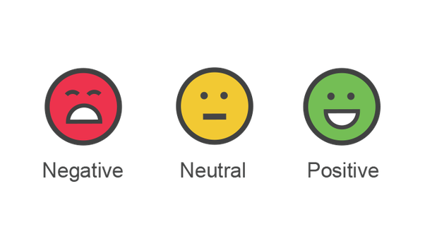
We will use the polarity_scores method to obtain the polarity indices for the given text and classifies each one in Positive, Neutral, or Negative.
The polarity score is the difference between these three categories, where -1 is the most extreme negative and +1 the extreme positive.
SIA = SentimentIntensityAnalyzer()

# Applying Model, Variable Creation
data['Polarity Score']=data["Review Clean"].apply(lambda x:SIA.polarity_scores(x)['compound'])

# Converting 0 to 1 Decimal Score to a Categorical Variable
data['Sentiment']=''
data.loc[data['Polarity Score']>0,'Sentiment']='Positive'
data.loc[data['Polarity Score']==0,'Sentiment']='Neutral'
data.loc[data['Polarity Score']<0,'Sentiment']='Negative'
df = data[['Review Text','Review Clean','Polarity Score','Sentiment']]
Word cloud of the positive and negatives words
Now that we have the reviews classified as Positive or Negative, we can take a look at the words that appear the most in the positive/negative reviews.
stop_words = set(STOPWORDS)
stop_words.update([x.lower() for x in list(data["Class Name"][data["Class Name"].notnull()].unique())] + ["dress", "petite", "skirt","shirt"])
def wordCloud(data, background_color, title):
    plt.figure(figsize = (10,10))
    wc = WordCloud(background_color = background_color, max_words = 500, stopwords = stop_words, max_font_size = 50)
    wc.generate(' '.join(data))
    plt.imshow(wc, interpolation="bilinear")
    plt.title(title)
    plt.axis('off')
positive_reviews = df[df['Sentiment'] == 'Positive']
wordCloud(positive_reviews['Review Clean'], 'white', "Most Used Words Positive Reviews")

negative_reviews = df[df['Sentiment'] == 'Negative']
wordCloud(negative_reviews['Review Clean'], 'black', "Most Used Words Negative Reviews")

4. Data preparation
In order to create our prediction model, we are going to need to prepare the data.
First of all, let's look at the distribution of the data according to its sentiment.
target_count = df['Sentiment'].value_counts()
print("Positive:",  target_count[0])
print("Negative:",  target_count[1])
print("Neutral:",  target_count[2])

plot_distributionCount('Sentiment',df)

We can see that the data is imbalanced. This can be a problem when we try to classify because the classifier could obtain 90% accuracy just by predicting always positive.
The solution of the imbalanced data is to use resampling techniques.
It consists of:
- Under-sampling: sampling from the majority class to keep only a part of these points.
- Over-sampling: replicating some points from the minority class.
- Generating synthetic data: creat new synthetic points from the minority class.
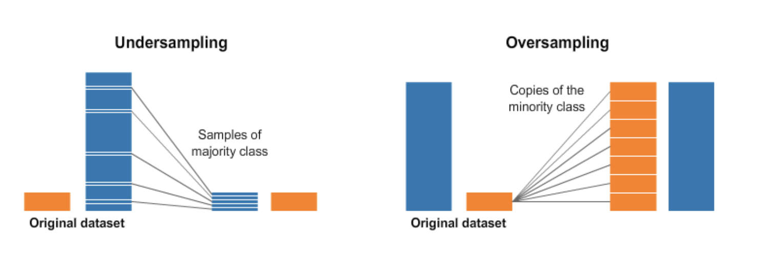
We will use the imblearn library, specifically the SMOTETomek class that combine over- and under-sampling. To know more you can check the documentation.
from imblearn.combine import SMOTETomek

smt = SMOTETomek(sampling_strategy='auto')
Now, we select the 'X' and the 'y' and split our entire data in two different sets:
- Train: used for training our model.
- Test: used for evaluating our model.
vectorizer = CountVectorizer()
# Choosing the X and Y where X is going to be the review text cleaned,
# Y is the label: the sentiment.
X = vectorizer.fit_transform(df['Review Clean'])
y = df['Sentiment']

# Fit the model
X_smt, y_smt = smt.fit_sample(X, y)

# Split the data into train and test
X_train, X_test, y_train, y_test = train_test_split(X_smt, y_smt, test_size=0.3, random_state=100)
5. Model creation
To achieve our objective and make possible to predict the sentiment of a clothing review, we are going to create four different models and compare them to see which one gives us the best results.
logisticRegression = LogisticRegression()
naiveBayes = MultinomialNB()
SVM = SVC()
randomForest = RandomForestClassifier(n_estimators=50)
neuralNetwork = MLPClassifier()

models = [logisticRegression, naiveBayes, SVM, randomForest, neuralNetwork]
conf_matrix = []
acc = []
reports = []

# For each model we are going to fit the model with the x_train and y_train.
for model in models:
    model.fit(X_train, y_train)

    # Predict
    predictions = model.predict(X_test)

    # Get the accuracy of the predictions that the model has made.
    accuracy = round(accuracy_score(y_test, predictions)*100)

    # Save the confusion_matrix for each model
    model_cm = confusion_matrix(y_test.values, predictions)

    # Save the classification_report for each model
    report = classification_report(y_test, predictions)

    conf_matrix.append(model_cm)
    acc.append(accuracy)
    reports.append(report)
model_accuracy = PrettyTable()

model_accuracy.add_column("Model", ['Logistic Regresion', 'Naive Bayes', 'SVM', 'Random Forest', 'Neural Network'])
model_accuracy.add_column("Accuracy", acc)
print(model_accuracy)
We will continue onward analyzing the Random Forest and Neural Network models more in-depth since they had the best accuracy score.
5.1. Confusion Matrix
A confusion matrix tells us how well a model performs on each of the classes we trained to predict.
So we are going to see the confusion matrix of the Random Forest and Neural Network.
def plot_confusionMatrix(conf_matrix):
    plt.figure(figsize=(15,12))

    plt.subplot(2,2,1)
    plt.title("Random Forest Confusion Matrix")
    sns.heatmap(conf_matrix[3], annot = True, cmap="OrRd", fmt='.0f', cbar=False);

    plt.subplot(2,2,2)
    plt.title("Neural Network Confusion Matrix")
    sns.heatmap(conf_matrix[4], annot = True, cmap="OrRd", fmt='.0f',cbar=False);

    plt.show()
plot_confusionMatrix(conf_matrix)

5.2. ROC Curve
In addition to looking at the accuracy score, in classification problems, we can count on ROC Curve (Receiver Operating Characteristics). It is one of the most important evaluation metrics for checking any classification model's performance.
It tells how much the model is capable of distinguishing between classes. When is higher the area under the AUC, better the model is...
randomForest_prob = randomForest.predict_proba(X_test)
neuralNetwork_prob = neuralNetwork.predict_proba(X_test)
skplt.metrics.plot_roc(y_test, randomForest_prob)
plt.title("Random Forest ROC Curves", fontsize=15)
plt.show()

skplt.metrics.plot_roc(y_test, neuralNetwork_prob)
plt.title("Neural Network ROC Curves", fontsize=15)
plt.show()


In the ROC curve the y-axis is TPR (True Positive Rate) and in the x-axis the FPR (False Positive Rate).
from sklearn.metrics import roc_auc_score
print("AUC score for Random Forest: ", round((roc_auc_score(y_test, randomForest_prob, multi_class='ovr')),2))
print("AUC score for Neural Network: ", round((roc_auc_score(y_test, neuralNetwork_prob, multi_class='ovr')),2))
As we see in the obtained ROC Curve, we have approximately 97% probability that the model will distinguish between the positive, neutral, or negative sentiment.
5.3. More metrics
Last but not least, let's take a look at other metrics that help analyze which model is better:
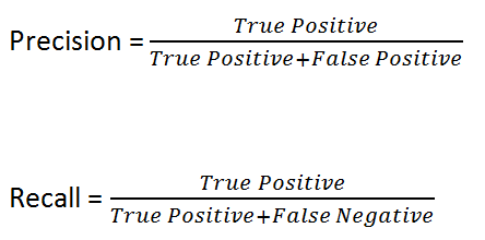
- Precision: Is the ability of a classifier not to label an instance positive that is negative.
- Recall: Is the ability of a classifier to find all positive instances.
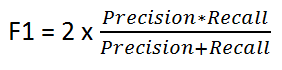
- F1-Score: This metric is needed when we want to seek a balance between Precision and Recall.
print("Random Forest Classification Report")
print(reports[3])
print("Neural Network Classification Report")
print(reports[4])
6. Conclusions
With all the results and the analysis, we have seen, we can expose the following conclusions:
- We have learned how to preprocess the text to solve a classification problem and how to determine the best model for our task.
- We have seen that most of the reviews are left by people between 30 and 50 years old approximately.
- We have also seen the different ways in which we can evaluate a classifier.
- Our two best models are working properly, as can be seen in the correlation matrix, the ROC Curves, and the precision, recall reports.