Introduction

This blog will provide an example of how to properly solve a problem where we need to get a regression function over some data distribution.

In this case I will be using this dataset from kaggle. It's a dataset that contains data about properties of the population from different countries and years.
For this set of population, it also provides the total number of people that match these conditions and the number of people that commited suicide.

So, the purpose for this dataset is to guess the number of suicides that happened given the information of the people.

For this project, I've tried different approaches, but the better results have come from a polynomial regressor, whose training code I will be explaining now.

Dependences

• pandas: vector and matrix operations
• numpy: extra functionality for pandas
• sklearn: to preprocess and split our data and train ML models
• matplotlib: using pyplot for pretty-plotting our results
• seaborn: also fancy plotting

import pandas as pd
import matplotlib.pyplot as plt
import numpy as np
import sklearn
import seaborn as sns

Missing values

We must take care of the missing values. To do this, we will check the number of missing values by column. This code will print the total number of samples and then print the missing values each column has.

dataset = pd.read_csv(r'data\master.csv')
print('Total original samples: ', len(dataset))
print(dataset.isna().sum(axis=0))

In this case, only the column "HDI_for_year" has missing values, and has too many of them (19456 over the 27820 total). Because it has too many of them, we will have to remove the column.

In fact, exploring the raw data, we see a column named "country-year", which contains the string concatenation of the country and the year. We will also remove this column because it's redundant information in a worse format for the model.

Finally, there is another column that must be removed for this problem. Not because there's any problem with the column, but because it is a column that we won't have when demanding a prediction.

del dataset['country-year']      # redundant
del dataset['HDI_for_year']      # unusable: too many missing values
del dataset['suicides/100k pop'] # the regressor must learn without this data

Data Modification

In order to use some columns, some transformation have to be done. There are 4 columns that hold categorical values and must be transformed into a numerical view in order to be used by the model. These would be "country", "sex", "age" and "generation".

# transform categorical to continuous
factorizables_mapping = {}
factorizable_names = ['country', 'sex', 'age', 'generation']
for fact_name in factorizable_names:
    dataset[fact_name], factorizables_mapping[fact_name] = pd.factorize(dataset[fact_name])

Also, the column "gdp_for_year_$" has a non-integer format despite representing one. It's because the number contains the thousands separator. Those would be commas. We need to transform it into an integer.

dataset['gdp_for_year_$'] = dataset['gdp_for_year_$'].str.replace(',', '')
dataset['gdp_for_year_$'] = pd.to_numeric(dataset['gdp_for_year_$'])

At last, we should shuffle the whole dataset in order to fully randomise the dataset splits and the training order.

# shuffle the dataset
dataset = dataset.sample(frac=1)

Data Analysis

Here are the finally used features:

• "country": the country the people is from
• "year": the year that this row inspects
• "sex": the sex of the people of this set
• "age": the age range
• "population": the number of people that there is in that set
• "gdp_foryear\$": the anual GDP of the country that year
• "gdp_percapita\$": the GDP per capita of the country that year
• "generation": the generation this person belongs to

And the target:

• "suicides_no": the number of suicides that happened in the population group

It's really important to check the correlations between your features in order to explore your data fully.

Here we can see the correlation between all the features.

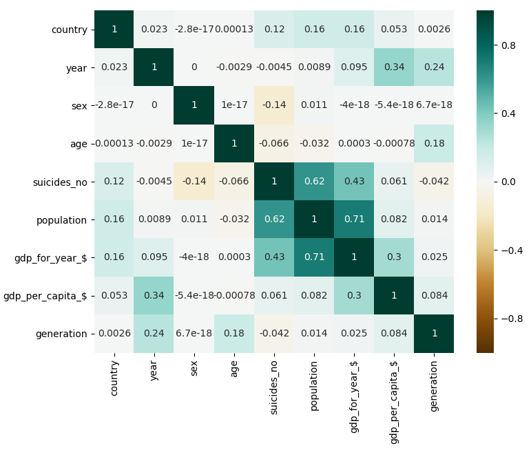
It has been generated by doing:

correlations = dataset.corr()

sns.heatmap(correlations, center=0, annot=True, vmin=-1, vmax=1, cmap="BrBG")
plt.show()

There are two correlations that stand out in the heatmap.

The first correlation is between the time scheduled for the plane departure and the time scheduled for the plane to arrive. This makes sense, because the arrival time will always depend on the departure time, specially for flights between airports of the United States.

The second correlation is between the origin airport and the destination airport. This makes sense, because the flights between some airports will be more common because of closeness and stops, for instance.

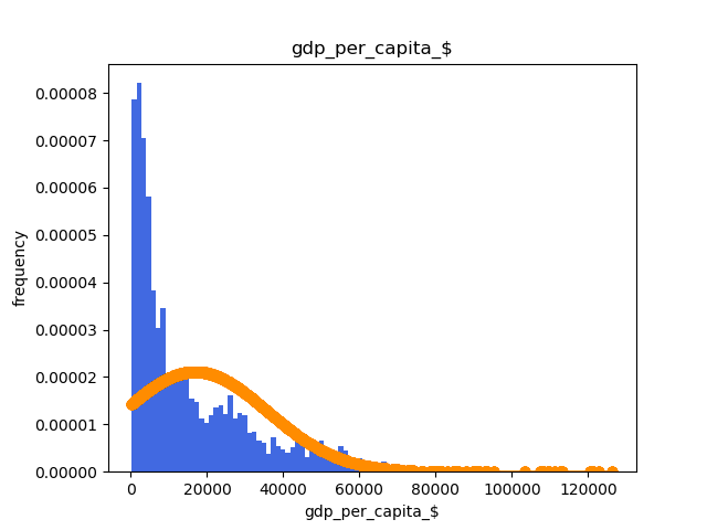
Also it's really important to check the data distribution. One of the usual tools to do this is the histogram per class. It's also important to check if the distribution follows a gaussian shape or not.

This can be done with the following code:

for column_name in dataset.columns:
    column_data = sorted(dataset[column_name])

    fit = stats.norm.pdf(column_data, np.mean(column_data), np.std(column_data))

    plt.title(column_name)
    plt.xlabel(column_name)
    plt.plot(column_data, fit, 'o-', color = "darkorange")
    plt.hist(column_data, color = "royalblue", density = True, bins=100)

    plt.show()

An histogram example is:

Data split

Now we will see how to split the dataset into a training and validation set. Because we always shuffle our data, this is simply getting the first N samples as the validation set and the rest as the train set.

val_prop = 0.2

num_entries = len(dataset)
num_entries_val = int(num_entries * val_prop)

x, y = get_xy(dataset) # function below

val_x = x.iloc[0:num_entries_val]
train_x = x.iloc[num_entries_val:]

val_y = y.iloc[0:num_entries_val]
train_y = y.iloc[num_entries_val:]

def get_xy(dataset):
    y = dataset['suicides_no']
    x = dataset.copy()
    del x['suicides_no']
    return x, y

Data Normalization

Data normalization is often recommended for training machine learning models.

Normalization implies reescalating the data so that the magnitude of the features doesn't affect the importance the algorithm gives it. For instance, imagine we have 2 features: "price" and "number of items". And let's say the number of items always goes from 1 to 5 and the price goes from 0 to 100. Our algorithm will probably take much more into account the feature "price" because of its magnitude. Well, normalization solves these problems.

I've implemented 2 types of normalization: MinMax and Standard. One uses the maximum and minimum values of the feature, and the other one uses the mean and standard deviation of the feature.

For me, in this problem, there was no difference in normalizing with one or another.

# DATA MINMAX NORMALIZATION (by sklearn)
# train_x
scaler = sklearn.preprocessing.MinMaxScaler()
train_x = scaler.fit_transform(train_x)

# val_x
val_x = scaler.transform(val_x)

# DATA MINMAX NORMALIZATION (own implementation)
# train_x
normalization_data = {}
maxs = [0] * len(train_x.columns)
mins = [0] * len(train_x.columns)

for index, feature_name in enumerate(dataset.columns):
    max_value = train_x[feature_name].max()
    min_value = train_x[feature_name].min()

    maxs[index] = max_value
    mins[index] = min_value

    if max_value == min_value:
        train_x[feature_name] = 0
    else:
        train_x[feature_name] = (train_x[feature_name] - min_value) / (max_value - min_value)

normalization_data['maxs'] = maxs
normalization_data['mins'] = mins

# val_x
for index, feature_name in enumerate(val_x.columns):
    max_value = normalization_data['maxs'][index]
    min_value = normalization_data['mins'][index]

    if max_value == min_value:
        val_x[feature_name] = 0
    else:
        val_x[feature_name] = (val_x[feature_name] - min_value) / (max_value - min_value)

# DATA STANDARD NORMALIZATION (by sklearn)
# train_x
scaler = sklearn.preprocessing.StandardScaler()
train_x = scaler.fit_transform(train_x)

# val_x
val_x = scaler.transform(val_x)

# DATA STANDARD NORMALIZATION (own implementation)
# train_x
normalization_data = {}
means = [0] * len(dataset.columns)
stds  = [0] * len(dataset.columns)

for index, feature_name in enumerate(dataset.columns):
    mean = dataset[feature_name].mean()
    std  = dataset[feature_name].std()

    means[index] = mean
    stds[index]  = std

    if std == 0:
        dataset[feature_name] = 0
    else:
        dataset[feature_name] = (dataset[feature_name] - mean) / std

normalization_data['means'] = means
normalization_data['stds'] = stds

# val_x
for index, feature_name in enumerate(dataset.columns):
    mean = normalization_data['means'][index]
    std = normalization_data['stds'][index]

    if std == 0:
        dataset[feature_name] = 0
    else:
        dataset[feature_name] = (dataset[feature_name] - mean) / std

Used Metrics

Because this is a regression problem, we will be using specific metrics to value our model.

• R^2 score: The R^2 coefficient scores how representative is the prediction made by the model compared with the real data. Normally, the coefficient takes a value between 0 and 1, being 1 a perfect representation of the data.

• Mean Squared Error (MSE): It corresponds to calculating the mean of all the errors squared. Error here means the difference between the predicted value and the correct value. This metric is one of the oldest and most used ones. Despite that, it is a very simple analysis and it's affected by the magnitude changes in the features. In top of that, because our calculations depend on a quadratic component, the results are not meaningful in an absolute way, but relative to other MSE evaluations.

• Root Mean Squared Error (RMSE): It's the square root of the MSE. This metric has the same properties as the previous one, except for that this one does give us the information in an absolute way. This is because we remove the quadratic component by doing the square root.

Model Training

Now we can finally train our model. In order to get a degree N polynomial regressor we need to create a "PolynomialFeatures" and a "LinearRegression" objects. The former will transform the original data in order to allow the latter to use it as if it were a degree 5 regressor.

To change the degree, it's enough to modify the variable "regression_degree".

regression_degree = 5

# generating model classes
poly_feat = sklearn.preprocessing.PolynomialFeatures(degree=regression_degree)
regressor = sklearn.linear_model.LinearRegression()

# fitting the [degree 5 to linear] model
poly_feat.fit(train_x, train_y)

# transforming both datasets to the linear space
poly_train_x = poly_feat.transform(train_x)
poly_val_x = poly_feat.transform(val_x)

# fitting the LinearRegressor to the training data
regressor.fit(poly_train_x, train_y)

# getting both train and val prediction
predicted_train_y = regressor.predict(poly_train_x)
predicted_val_y  = regressor.predict(poly_val_x)

# computing the MSE for both
train_MSE = np.mean(np.square(predicted_train_y - train_y))
val_MSE  = np.mean(np.square(predicted_val_y - val_y))

# computing the RMSE for both
train_RMSE  = np.sqrt(train_MSE)
val_RMSE  = np.sqrt(val_MSE)

# computing the R^2 score for both
train_r2_score = sklearn.metrics.r2_score(train_y, predicted_train_y)
val_r2_score = sklearn.metrics.r2_score(val_y, predicted_val_y)

print('Train Score: "{}"'.format(train_r2_score))
print('Validation Score: "{}"'.format(val_r2_score))

print('Train MSE: "{}"'.format(train_MSE))
print('Validation MSE: "{}"'.format(val_MSE))

print('Train RMSE: "{}"'.format(train_RMSE))
print('Validation RMSE: "{}"'.format(val_RMSE))

After some trial and error with the polynome degree, I composed this plot. It shows the evolution of the R^2 score and the MSE when variating the degree of the polynome for both the train and validation set.

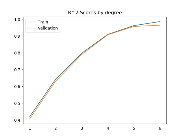
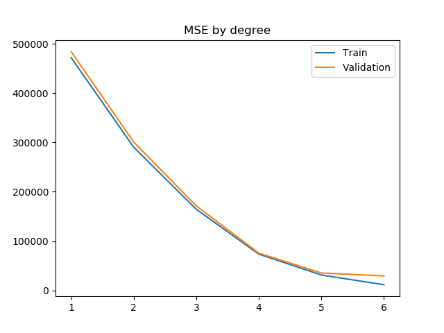
These two plots show a very interesting point of Machine Learning: overfitting.

Generally, by raising the degree of the polynome, the regressor can get a more fitting model to the data that it's been given. This means that it will give better and better results for the train set.

However, the more fitted it becomes to the train set, the less accurate it becomes with the data it hasn't been exposed to during the train phase, because this new data doesn't follow the exact distribution of the original one.

This becomes apparent with this plot. We can see that the validation R^2 score raises following the training R^2 score until degree 5. With the degree 6, we can see that the R^2 score and the MSE stop improving. This is why we will choose degree 5 for our model.